Home
/
Analysis
/
Joint Analysis
Functional Enrichment
Clustering Analysis
Download
/
Help
Machine Learning
Overview
Step1: Data Input
Step2: Method Selection
Step3: Model Generation
Step4: Feature Browse
Step5: Model Evaluation
Step6: Model Application
Next Step
Basic Parameter
*
Analysis Type:
Binary Classification
Multiple Classification
Survival Analysis
*
The generation way for validation set:
Upload Dataset
Divide Dataset
*
Missing Value Treatment:
Delete Rows
Fill by Mean
Fill by Median
Fill by Maximum
Fill by Minimum
Fill by Mode
Data Set
*
Upload Matrix File:
*
Upload Group Information File:
*
Proportion of Division: training : validation =
7 : 3
Training Set
*
Upload Matrix File:
*
Upload Group Information File:
Validation Set
*
Upload Matrix File:
*
Upload Group Information File:
Please make sure the input file format is correct to avoid errors that caused no results.
The contents of the files should be separated by tab.
In the upload matrix file, each line should be a feature and each column should be a sample. Features and samples can not be repeated, otherwise there is no result.
If the group information file do not contain survival information, MLBiomarker will perform analysis of "Binary/Multi-class", the file header should be "sample", "condition". Samples of the same condition should be placed together, not out of order. The value of the "condition" for binary-class should be "case" or "control".
If the group information file contains survival information, MLBiomarker will perform "Survival Analysis", the file header should be "sample", "time" and "status". The value of the "status" should be "0" or "1".
The feature ID and sample ID should not contain special characters. Otherwise, underline will be used instead.
Too many features and samples will result in slow running time.
In the results, the higher the "importance score", the more important the feature; The lower the "avgrank", the more important the feature.
If some ML methods do not produce results of "Biomarker Identification" or "Biomarker Evaluation", users are advised to adjust the parameters and try again.
In the form below, click the button of "parameter" can adjust the parameters of the corresponding ML method.
Submit
Last Step
Method Selection
Next Step
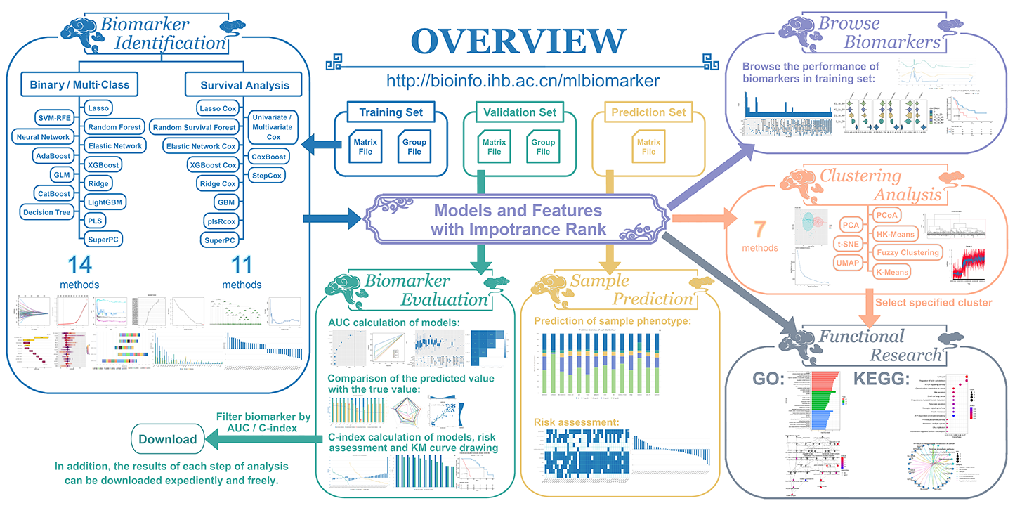
"Biomarker Identification" involves two kinds of analysis: "Binary/Multi-class" and "Survival Analysis". The former is oriented towards biclassification and multi-classification biological events, and MLBiomarker has 14 corresponding analysis methods to choose from. The latter is oriented towards survival analysis, and MLBiomarker has 11 corresponding analysis methods to choose from.
Some ML methods are time-consuming, please be patient. The method selected in the form below is the one that runs faster.
After users perform an analysis of the "Biomarker Identification", a floating navigation bar will appear in the upper right corner of the results page for the analysis of the other three sections.
In the results of each ML method, the number of identified biomarkers could be adjusted according to the important scores. At the end of the results, At the end of the results, users can download and browse the intersection of these top biomarkers.
After users perform an analysis of the "Biomarker Identification", a floating navigation bar will appear in the upper right corner of the results page for the analysis of the other four sections.
Algorithm and Parameter Selection
Select All
Lasso
parameter
introduction
hide
Model:
binomial
gaussian
poisson
Cross Validation:
fold
Show the top
biomarkers
Compared with the quadratic penalty function of ridge regression, lasso's first penalty function can not only shrink the non-0 predictors βj to 0, but also select the valuable predictors (|βj| with a large value). This is because compared with the quadratic penalty function of ridge regression, lasso's first penalty function has a smaller contraction degree on the variable coefficient port βj, so lasso can select a more accurate model.
Detail.
Elastic Network
parameter
introduction
hide
Model:
binomial
gaussian
poisson
Cross Validation:
fold
Alpha:
0.
Show the top
biomarkers
The penalty function of the elastic network is a convex linear combination of the ridge regression penalty function and the Lasso penalty function. When α=0, elastic network regression is ridge regression. When α=1, elastic network regression is lasso regression. Therefore, elastic net regression has the advantages of lasso regression and ridge regression, which can not only achieve the purpose of variable selection, but also have a good group effect.
Detail.
Ridge
parameter
introduction
hide
Model:
binomial
gaussian
poisson
Cross Validation:
fold
Show the top
biomarkers
Ridge regression is a biased estimation regression method dedicated to collinear data analysis. In fact, it is an improved least squares estimation method. By giving up the unbias of least squares method, Ridge regression can obtain a regression method with more realistic and reliable regression coefficient at the cost of losing some information and reducing accuracy. The fit of ill-conditioned data is better than the least square method.
Detail.
XGBoost
parameter
introduction
hide
Model:
Eta: 0.
Max depth:
Objective:
binary:logistic
multi:softmax
count:poisson
The number of decision trees to display:
Show the top
biomarkers
Extreme Gradient Boosting, which is an efficient implementation of the gradient boosting framework from Chen & Guestrin (2016). XGBoost includes efficient linear model solver and tree learning algorithms. The package can automatically do parallel computation on a single machine which could be more than 10 times faster than existing gradient boosting packages. It supports various objective functions, including regression, classification and ranking. The package is made to be extensible, so that users are also allowed to define their own objectives easily.
Detail.
PLS
parameter
introduction
hide
Show the top
biomarkers
PLS (partial least squares) regression uses the principle of principal component analysis to condense multiple X and multiple Y into components (X corresponds to principal component U, Y corresponds to principal component V), and then with the help of the typical correlation principle, the relationship between X and U, Y and V can be analyzed. And combined with the principle of multiple linear regression, analyze the relationship between X and V, so as to study the relationship between X and Y.
Detail.
Decision Tree
parameter
introduction
hide
Show the top
biomarkers
A decision tree models the decision logics i.e., tests and corresponds outcomes for classifying data items into a tree-like structure. The nodes of a DT tree normally have multiple levels where the first or top-most node is called the root node. All internal nodes (i.e., nodes having at least one child) represent tests on input variables or attributes. Depending on the test outcome, the classification algorithm branches towards the appropriate child node where the process of test and branching repeats until it reaches the leaf node. The leaf or terminal nodes correspond to the decision outcomes. When traversing the tree for the classification of a sample, the outcomes of all tests at each node along the path will provide sufficient information to conjecture about its class.
Neural Network
parameter
introduction
hide
Model:
Hidden:
Activation Function:
logistic
tanh
Algorithm:
rprop+
rprop-
backprop
sag
slr
Show the top
biomarkers
Neural networks (NN) attempt to use multiple layers of calculations to imitate the concept of how the human brain interprets and draws conclusions from information. NN are essentially mathematical models which are designed to deal with complex and disparate information, and the nomenclature of this algorithm comes from its use of 'nodes' akin to synapses in the brain. The learning process of a NN can either be supervised or unsupervised. A neural net is said to learn in a supervised manner if the desired output is already targeted and introduced to the network by training data whereas unsupervised NN have no such preidentified target outputs and the goal is to group similar units close together in certain areas of the value range. The process of learning used in MLBiomarker is supervised.
Detail.
SVM-RFE
parameter
introduction
hide
Cross Validation:
K fold:
N fold:
Show the top
biomarkers
SVM (support vector machine) first maps each data item into an n-dimensional feature space where n is the number of features. It then identifies the hyperplane that separates the data items into two classes while maximising the marginal distance for both classes and minimising the classification errors. The marginal distance for a class is the distance between the decision hyperplane and its nearest instance which is a member of that class. More formally, each data point is plotted first as a point in an n-dimension space (where n is the number of features) with the value of each feature being the value of a specific coordinate. To perform the classification, we then need to find the hyperplane that differentiates the two classes by the maximum margin.
Detail.
GLM
parameter
introduction
hide
Model:
binomial (Logistic Regression)
gaussian (Linear Regression)
poisson (Poisson Regression)
Show the top
biomarkers
In GLM (generalized linear model), logistic regression is used for analysis of binary-class, linear regression is used for analysis of multi-class.
Detail.
LightGBM
parameter
introduction
hide
Model:
Learning Rate: 0.
Objective:
binary
multiclass
Show the top
biomarkers
LightGBM is a gradient boosting framework that uses tree based learning algorithms. It is designed to be distributed and efficient with the following advantages:
Faster training speed and higher efficiency.
Lower memory usage.
Better accuracy.
Support of parallel, distributed, and GPU learning.
Capable of handling large-scale data.
For further details, please refer to Features.
Benefiting from these advantages, LightGBM is being widely-used in many winning solutions of machine learning competitions.
Comparison experiments on public datasets show that LightGBM can outperform existing boosting frameworks on both efficiency and accuracy, with significantly lower memory consumption. What's more, distributed learning experiments show that LightGBM can achieve a linear speed-up by using multiple machines for training in specific settings.
Detail.
CatBoost
parameter
introduction
hide
Model:
Number of iterations:
Loss function:
Logloss
MultiClass
Show the top
biomarkers
CatBoost is a fast, scalable, high performance gradient boosting on decision trees library. Used for ranking, classification, regression and other ML tasks.
Detail.
AdaBoost
parameter
introduction
hide
Number of iterations:
Show the top
biomarkers
M1 algorithm and Breiman's Bagging algorithm using classification trees as individual classifiers. Once these classifiers have been trained, they can be used to predict on new data. Also, cross validation estimation of the error can be done.
Detail.
SuperPC
parameter
introduction
hide
Show the top
biomarkers
Does prediction in the case of a censored survival outcome, or a regression outcome, using the "supervised principal component" approach (Bair et al., 2006).
Superpc is especially useful for high-dimensional data when the number of features p dominates the number of samples n (p >> n paradigm), as generated, for instance, by high-throughput technologies.
Detail.
Random Forest
parameter
introduction
hide
Number of Trees:
Random forest (RF) is an ensemble classifier and consisting of many DTs (decision trees) similar to the way a forest is a collection of many trees. DTs that are grown very deep often cause overfitting of the training data, resulting a high variation in classification outcome for a small change in the input data. They are very sensitive to their training data, which makes them error-prone to the test dataset. The different DTs of an RF are trained using the different parts of the training dataset. To classify a new sample, the input vector of that sample is required to pass down with each DT of the forest. Each DT then considers a different part of that input vector and gives a classification outcome. The forest then chooses the classification of having the most 'votes' (for discrete classification outcome) or the average of all trees in the forest (for numeric classification outcome). Since the RF algorithm considers the outcomes from many different DTs, it can reduce the variance resulted from the consideration of a single DT for the same dataset.
Detail.
Lasso Cox
parameter
introduction
hide
Model:
cox
Cross Validation:
fold
Show the top
biomarkers
Compared with the quadratic penalty function of ridge regression, lasso's first penalty function can not only shrink the non-0 predictors βj to 0, but also select the valuable predictors (|βj| with a large value). This is because compared with the quadratic penalty function of ridge regression, lasso's first penalty function has a smaller contraction degree on the variable coefficient port βj, so lasso can select a more accurate model.
Detail.
Elastic Network Cox
parameter
introduction
hide
Model:
cox
Cross Validation:
fold
Alpha:
0.
Show the top
biomarkers
The penalty function of the elastic network is a convex linear combination of the ridge regression penalty function and the Lasso penalty function. When α=0, elastic network regression is ridge regression. When α=1, elastic network regression is lasso regression. Therefore, elastic net regression has the advantages of lasso regression and ridge regression, which can not only achieve the purpose of variable selection, but also have a good group effect.
Detail.
Ridge Cox
parameter
introduction
hide
Model:
cox
Cross Validation:
fold
Show the top
biomarkers
Ridge regression is a biased estimation regression method dedicated to collinear data analysis. In fact, it is an improved least squares estimation method. By giving up the unbias of least squares method, Ridge regression can obtain a regression method with more realistic and reliable regression coefficient at the cost of losing some information and reducing accuracy. The fit of ill-conditioned data is better than the least square method.
Detail.
XGBoost Cox
parameter
introduction
hide
Model:
Eta: 0.
Max depth:
Objective:
survival:cox
The number of decision trees to display:
Show the top
biomarkers
Extreme Gradient Boosting, which is an efficient implementation of the gradient boosting framework from Chen & Guestrin (2016). XGBoost includes efficient linear model solver and tree learning algorithms. The package can automatically do parallel computation on a single machine which could be more than 10 times faster than existing gradient boosting packages. It supports various objective functions, including regression, classification and ranking. The package is made to be extensible, so that users are also allowed to define their own objectives easily.
Detail.
plsRcox
parameter
introduction
hide
Model:
Number of Components:
Cross Validation:
fold
Show the top
biomarkers
Too high number of components may result in no result.
plsRcox implements partial least squares Regression and various regular, sparse or kernel, techniques for fitting Cox models in high dimensional settings. Cross validation criteria were studied in Bertrand's research.
Detail.
StepCox
parameter
introduction
hide
Model:
bidirection
forward
backward
Show the top
biomarkers
Stepwise regression is a method of fitting regression models in which the choice of predictive variables is carried out by an automatic procedure. Three stepwise regression can be chosen, i.e. stepwise linear regression, stepwise logistic regression and stepwise cox regression.
Detail.
GBM
parameter
introduction
hide
Model:
Number of trees:
Learning rate (0.001~0.1):
Show the top
biomarkers
Too small dataset may result in no result.
A smaller learning rate typically requires more trees.
GBM (Gradient Boosting Machine) algorithm is one of Boosting algorithm. The main idea is that multiple weak learners are generated serially, and the goal of each weak learner is to fit the negative gradient of the loss function of the previously accumulated model so that the cumulative model loss after adding the weak learner decreases in the direction of the negative gradient. And it combines the base learners linearly with different weights, so that the excellent learners can be reused. The most common base learner is the tree model.
Detail.
CoxBoost
parameter
introduction
hide
Show the top
biomarkers
CoxBoost provides routines for fitting Cox models by likelihood based boosting for a single endpoint or in presence of competing risks.
Detail.
SuperPC
parameter
introduction
hide
Show the top
biomarkers
Does prediction in the case of a censored survival outcome, or a regression outcome, using the "supervised principal component" approach (Bair et al., 2006).
Superpc is especially useful for high-dimensional data when the number of features p dominates the number of samples n (p >> n paradigm), as generated, for instance, by high-throughput technologies.
Detail.
Random Survival Forest
parameter
introduction
hide
Number of Trees:
Random survival forest (RSF) is a random forest method for analyzing right censored survival data. It introduces new survival splitting rules for growing survival trees, and new missing data algorithms for estimating missing data.
RSF introduced the event retention principle for surviving forests and used it to define overall mortality, a simple interpretable mortality measure that can be used to predict outcomes.
Detail.
Cox
(Univariate / Multivariate)
parameter
introduction
hide
Model:
(Univariate Cox) P value < 0.
(Multivariate Cox) P value < 0.
Show the top
biomarkers
The main purpose of survival analysis is to study the relationship between covariate (independent variable) X and the observed survival function S(t,X). When S(t,X) is affected by covariate, the traditional method is to consider regression analysis, that is, the influence of various covariables on S(t,X). Because the survival data contains truncated data, it is difficult to solve the above problems with general regression analysis. A very important content of survival analysis is to explore the risk factors affecting survival time or survival rate, which can affect the survival rate by affecting the risk of death at various times (that is, the risk rate). The risk rate function of different populations at different times is different, and the risk rate function is usually expressed as the product of the baseline risk rate function and the corresponding covariate function. In 1972, British biostatistician D. Cox proposed a method for estimating model parameters when the baseline risk rate function was unknown. Later generations called this model Cox proportional risk regression model, referred to as Cox regression.
Detail.
Last Step
Model Generation
Next Step
Lasso
Elastic Network
Ridge
XGBoost
PLS
Decision Tree
Neural Network
SVM-RFE
GLM
LightGBM
CatBoost
AdaBoost
SuperPC
Random Forest
Lasso Cox
Elastic Network Cox
Ridge Cox
XGBoost Cox
plsRcox
StepCox
GBM
CoxBoost
SuperPC
Random Survival Forest
Cox
Lasso
Elastic Network
Ridge
XGBoost
PLS
Decision Tree
Neural Network
SVM-RFE
GLM
LightGBM
CatBoost
AdaBoost
SuperPC
Random Forest
Lasso Cox
Elastic Network Cox
Ridge Cox
XGBoost Cox
plsRcox
StepCox
GBM
CoxBoost
SuperPC
Random Survival Forest
Cox
Last Step
Feature Browse
Next Step
Last Step
Model Evaluation
Next Step
Last Step
Model Application
Next Step
Last Step
copyright 2025-present@The Quzhou Affiliated Hospital of Wenzhou Medical University, Quzhou People's Hospital